Walkthrough of TensorFlow Architecture
- Software engineering
TensorFlow is one of the most popular libraries in the modern Machine Learning ecosystem. It provides functionality for users to easily build, train and deploy deep learning models with its high-level Python API. At G-Research, we’re more than just users of TensorFlow. We require an understanding of its inner workings in order to support our researchers in developing cutting edge deep learning models and to extend its functionality to suit our specific needs. This blog post provides an introduction to TensorFlow’s architecture, aimed at TensorFlow users who are interested in diving into the source code, just as we did.
Anatomy of a Tensor
Tensors are the most fundamental objects in any TensorFlow program and will be familiar to any TensorFlow user. At its core, a tensor is a contiguous block of memory with associated data type and shape metadata that represents a multi-dimensional array. It can store no more than 254 dimensions and is represented in memory in a row-major format, as shown in Figure 1.
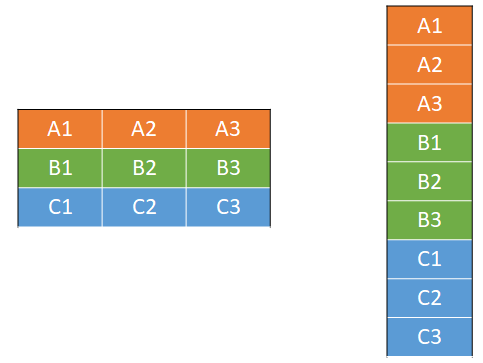
Figure 1: Row-major representation of a tensor.
The core tensor object is defined in tensorlow/core/framework/tensor.h
and is a thin wrapper around the Eigen Tensor, where Eigen is a header-only C++ linear algebra library that is used heavily throughout TensorFlow and is highly optimised for performance. Many of the CPU versions of linear algebra operations within TensorFlow are just calls to the Eigen equivalent or rely on functions from Eigen to implement the behaviour (see examples in tensorflow/core/kernels).
Tensor Indexing
Since tensors are row-major and contain just a single data type, the type and shape metadata can be used to index into a tensor by calculating the required location in memory and jumping there directly. For example, consider the 2-dimensional, shape (2, 3), type tf.int32 tensor show in Figure 2 below, along with its row-major memory block.
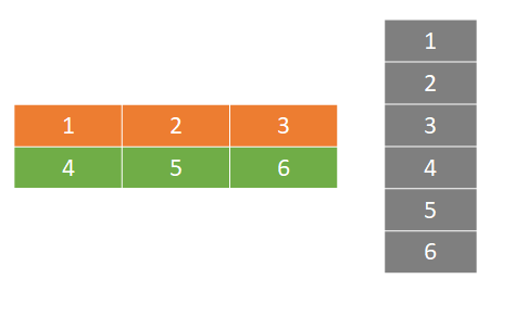
Figure 2: A two-dimensional (2, 3) int32 tensor.
Retrieving the element at position [1, 2] requires moving forward 1 * 12 bytes to get to the required row (3 elements per row times 4 bytes per int32 element), followed by an additional 2 * 4 bytes to get to the required column.
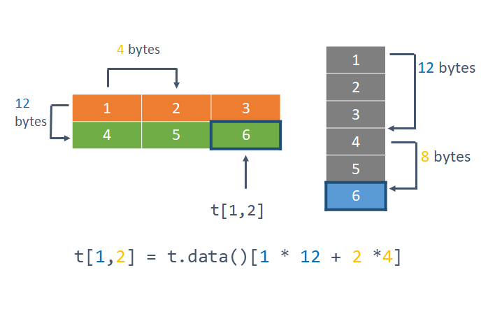
Figure 3: Indexing into a 2-dimensional tensor using the type and shape metadata.
Tensor Slicing
In addition to shape and type metadata, NumPy arrays also contain strides metadata. This is just a tuple describing the number of bytes to step in each dimension in order to reach the next element in that dimension. If we convert the above tensor to a NumPy array with .numpy(), we can inspect the strides property, which reveals that we must step 12 bytes to access the next element in the first (row) dimension and 4 bytes to access the next element in the second (column) dimension.
t = tf.constant([[1, 2, 3], [4, 5, 6]])
arr = a.numpy()
a.strides

>>> (12, 4)
This strides metadata allows you to slice any dimension of a NumPy array and return a view rather than a copy of the original data – the strides metadata of the resulting array is changed, and it may no longer be a contiguous block in memory. By contrast, TensorFlow tensors do not contain strides metadata. They must be represented as contiguous blocks in memory in order to allow indexing, which means that slicing a TensorFlow tensor will always create a copy unless you slice the first dimension.
TensorFlow Graphs and Operations
When a user defines a neural network, loss function and optimiser in TensorFlow, it gets represented as a graph defining the computations the user wishes to execute. The nodes in the graph are operations (or “ops”) that define the mathematical operations that manipulate tensors and the edges in the graph are the tensors that “flow” from one op to another (hence the name TensorFlow!).
Operations take 0 or more tensors as input and produce 0 or more tensors as output. The backbone of every op is its Compute method that determines what the op does with the input tensors to generate the output tensors and this is normally implemented in C++ and/or CUDA. Ops typically have an explicit, corresponding gradient op which takes the gradients of the original op’s outputs as input and returns the gradients with respect to the op’s inputs.
Graph Mode vs Eager Execution
Since TensorFlow 2.0 was released in 2019, the default execution mode has been eager execution. This means when you execute a TensorFlow operation, you receive the result back in Python immediately as shown in the code example below. Eager execution makes writing and debugging TensorFlow code much simpler.
x = [[2.]]
m = tf.matmul(x, x)

# Result of the matmul is returned immediately in Python
>> [[4.]]
Prior to TensorFlow 2.0, the default execution mode was graph mode, in which the user first defines their TensorFlow graph with the ops they would like to execute and then feeds data into this graph at runtime. The equivalent example in TF1.x is shown below for illustrative purposes. Note how this includes a tf.placeholder object x which defines a parameter to be fed into the graph, where the actual value of x is specified at runtime as part of the feed_dict argument to sess.run.
# Define the input "placeholder" data to the computation graph and the operations that should be run
x = tf.placeholder(tf.float32)
mul = tf.matmul(x, x)

# Run the operations on some data i.e. feed data into the computation graph
with tf.Session() as sess:
    m = sess.run(mul, feed_dict={x: [[2.]]})

>> [[4.]]
TensorFlow 2.x still allows graph mode execution as it can offer better performance and enable use of TensorFlow models in environments without an available Python interpreter, such as mobile applications. Using the tf.keras model.fit and model.predict functionality will use graph execution unless it is explicitly disabled with the run_eagerly=True argument to model.compile.
TensorFlow 2.x also includes a tf.autograph library that converts Python and TensorFlow code to a TensorFlow graph. The tf.function decorator can be used to convert a Python function into a graph.
TensorFlow Compute Model – Graph Construction and Execution
In order to describe how TensorFlow executes a graph mode computation, let’s start with a simple TensorFlow implementation of a Dense layer and mean squared error loss.
@tf.function
def dense_layer_and_mse(x, y):
    z = tf.matmul(X, W)
    y_pred = tf.add(z, b)
    sq_diff = tf.math.squared_difference(y, y_pred)
    mse = tf.reduce_mean(sq_diff)
    return mse


# Dense layer weights and biases
W = tf.Variable(tf.random.normal([10, 1], stddev=0.1, dtype=tf.float32))
b = tf.Variable(tf.zeros([1, ], dtype=tf.float32))

# Random batch of inputs and labels
X = tf.random.normal([128, 10])
y = tf.random.normal([128, 1])

mse = dense_layer_and_mse(X, y)
TensorFlow represents the user’s network as a graph that looks something like Figure 4.
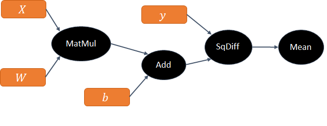
Figure 4: Graph for the forward pass.
In order to execute the operations in the correct order, TensorFlow performs a topological sort of the computation graph. This is an ordering of the nodes in a directed acyclic graph (DAG) such that for every directed edge between node U and node V, node U appears before V in the ordering. TensorFlow uses this ordering when it comes to execute the graph, ensuring for example that the result of the initial tf.matmul is available before the tf.add.
Next, TensorFlow takes the corresponding gradient op for each node in the forward pass and uses this to construct the appropriate backward graph. These two are then chained together to produce the full graph, as shown in Figure 5 below. Note how TensorFlow does not derive any gradients from the code – a full backward graph is created and each op has a corresponding, explicitly defined, gradient op.

Figure 5: Backward graph construction.
At the stage of backward graph construction, TensorFlow may insert additional ops into the backward graph in order to compute the required gradients that do not have an analogous op in the forward pass. This is best illustrated with a toy example. Figure 6 shows an op Op0 that broadcasts its output tensor z0 to three further ops, Op1, Op2 and Op3, which produce corresponding output tensors. To compute the gradient of any loss function L with respect to the input variable z0, the gradients must be summed as shown in the equation below.
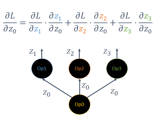
Figure 6: A single op’s output can be used as the input to multiple ops.
This requires TensorFlow to add an additional SumGradients operation to the backward graph, which clearly does not have an analogous op in the forward pass.
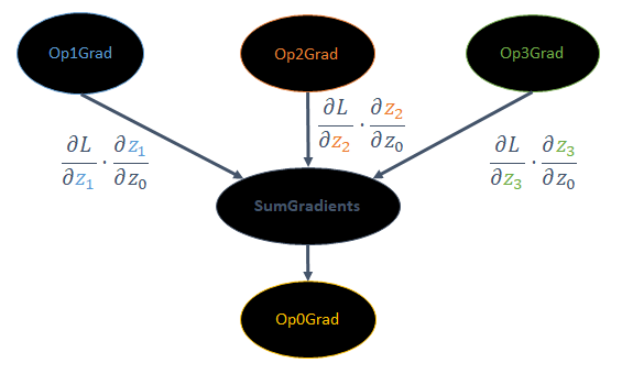
Figure 7: TensorFlow adds a SumGradients op as required by the chain rule.
Finally, once the full graph has been created, TensorFlow can step through each operation in the graph (in the order defined by the topological sort) and call the Compute method of each op to produce the final output tensor(s), which are then returned to the user in Python.
TensorFlow Graph Optimisations
As previously mentioned, running TensorFlow in graph mode can lead to performance improvements. TensorFlow contains a graph optimisation system called Grappler which applies various high-level operations to enable faster compute times and reductions in memory usage. “Op fusion” (or “Remapper Optimizer” as it’s referred to in the TensorFlow docs) is one of the many optimisations that can be applied. This fuses kernels for multiple operations into larger “monolithic” kernels, which can lead to performance improvements as there is less overhead from multiple GPU kernel launches. An example is fusing the common Matmul + BiasAdd + Activation pattern that is used frequently in feed-forward neural networks.
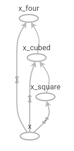
In practice, there are some cases where Grappler does not fuse operations despite a simpler implementation being available. Consider the very simple example below which uses two different ways of computing the fourth power of a tensor. The first method naively uses tf.multiply repeatedly while the second uses tf.math.pow(x, 4) directly. The TensorBoard computation graphs produced from these two methods are shown in the figures below.
We run the unfused_power_four function in both eager mode and graph mode (i.e. with and without the tf.function decorator) and use the Nvidia Visual Profiler to see which kernels are actually launched on the GPU, as shown in Table 1 below. The graph mode implementation trades an Eigen scalar_product_op for a scalar_square_op but otherwise still launches three kernels and does not fuse into a single kernel corresponding to tf.math.pow(x, 4).
@tf.function
def unfused_power_four(x):
    x_squared = tf.multiply(x, x, name="x_square")
    x_cubed = tf.multiply(x, x_squared, name="x_cubed")
    x_four = tf.multiply(x, x_cubed, name="x_four")
    return x_four


@tf.function
def power_four(x):
    return tf.math.pow(x, 4)
Figure 8: Unfused power four TensorBoard graph.
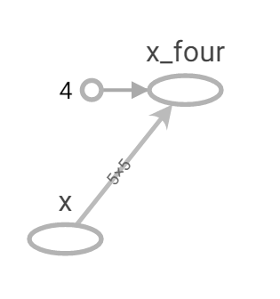
Figure 9: tf.pow TensorBoard graph
| Implementation | Kernel type | Number times launched |
|---|---|---|
| Graph Mode | ||
| Eigen::internal::scalar_product_op | 2 | |
| Eigen::internal::scalar_square_op | 1 | |
| Eager Mode | ||
| Eigen::internal::scalar_product_op | 3 |
Table 1: GPU kernel launches for power four example.
While this is just a toy example, the general point is important for real-world scenarios too. Consider implementing by hand the Gaussian Error Linear Unit (GELU) used in Google’s BERT language model. This can easily be implemented using basic TensorFlow operations such as tensor adds, multiplies, and special functions. Inspecting the graph constructed by TensorFlow in Figure 10, it is evident there are five element-wise tensor operations involved in the computation. Again, comparing the GPU kernel launches between eager execution and graph mode reveals that the same five kernels are launched in both cases.
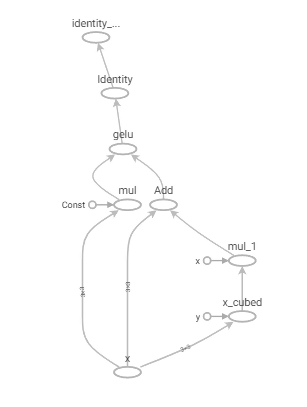
Figure 10: Hand implemented GELU TensorBoard graph.
To fuse operations in these cases, we must either implement the CUDA kernel for the operation ourselves or try a compiler such as XLA, which compiles the TensorFlow graph into a series of computation kernels specific to the model. This can also result in fewer, fused GPU kernels. XLA can be enabled by setting an environment variable or controlled more explicitly by passing the jit_compile=True argument to the tf.function decorator.
While XLA can give performance improvements in some scenarios, there are still times when it’s beneficial to write TensorFlow custom ops by hand, whether it’s to fuse operations, reduce memory usage, or implement functionality that does not exist in the library.
Check out our follow up blog post to learn how to write your own custom TensorFlow op from scratch!

